Capacity Planning#

Problem statement (interviewer prompt)

Estimate server count, storage, and bandwidth for a chat app with 200M MAU and 30 messages/user/day. Walk through user → QPS → storage → bandwidth → server count. Add 30% headroom and explain Little's Law in passing.

flowchart LR
  R([Requirements<br/>users / QPS / data size])
  L([Little's Law<br/>L = λ · W])
  N([Numbers every dev knows<br/>SSD, RAM, network])
  E([Estimate])
  H([Headroom 30 percent])
  R --> L --> E
  N --> E --> H

  classDef p fill:#dbeafe,stroke:#1e40af,stroke-width:1px,color:#0f172a;
  classDef s fill:#fef3c7,stroke:#92400e,stroke-width:1px,color:#0f172a;
  class R,H p;
  class L,N,E s;

    classDef client fill:#dbeafe,stroke:#1e40af,stroke-width:1px,color:#0f172a;
    classDef edge fill:#cffafe,stroke:#0e7490,stroke-width:1px,color:#0f172a;
    classDef service fill:#fef3c7,stroke:#92400e,stroke-width:1px,color:#0f172a;
    classDef datastore fill:#fee2e2,stroke:#991b1b,stroke-width:1px,color:#0f172a;
    classDef cache fill:#fed7aa,stroke:#9a3412,stroke-width:1px,color:#0f172a;
    classDef queue fill:#ede9fe,stroke:#5b21b6,stroke-width:1px,color:#0f172a;
    classDef compute fill:#d1fae5,stroke:#065f46,stroke-width:1px,color:#0f172a;
    classDef storage fill:#e5e7eb,stroke:#374151,stroke-width:1px,color:#0f172a;
    classDef external fill:#fce7f3,stroke:#9d174d,stroke-width:1px,color:#0f172a;
    classDef obs fill:#f3e8ff,stroke:#6b21a8,stroke-width:1px,color:#0f172a;
    class R,L,N,E,H service;

Capacity planning = "how big does it have to be?". The interview version is back-of-envelope estimation: from user count → QPS → storage → bandwidth → server count, in 5 minutes, before drawing boxes.

Numbers every developer should know#

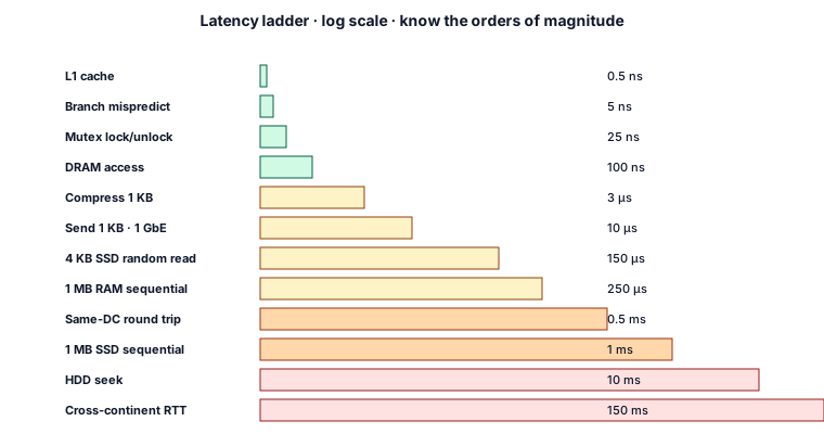
Operation	Time
L1 cache reference	0.5 ns
Branch mispredict	5 ns
L2 cache reference	7 ns
Mutex lock/unlock	25 ns
Main memory reference	100 ns
Compress 1 KB with Zippy	3,000 ns (3 µs)
Send 1 KB over 1 Gbps net	10,000 ns (10 µs)
Read 4 KB random from SSD	150,000 ns (150 µs)
Read 1 MB sequential from RAM	250,000 ns
Round trip in same DC	500,000 ns (0.5 ms)
Read 1 MB sequential from SSD	1,000,000 ns (1 ms)
HDD seek	10,000,000 ns (10 ms)
Cross-continent round trip	150,000,000 ns (150 ms)

(Memorise the orders of magnitude. Interviewers test the gap between RAM and disk a lot.)

Common throughput envelopes#

Resource	Order of magnitude
One commodity server CPU	~100k simple req/s
10 GbE NIC	~1 GB/s (8 Gbps usable)
NVMe SSD	1-7 GB/s, 1M IOPS
Postgres single primary	5-20k writes/s, much more reads via replicas
Redis single node	100k-1M ops/s
Kafka partition	10 MB/s comfortably
One WS gateway	100k concurrent conns

Little's Law#

L = λ · W

L = concurrent items in system.
λ = arrival rate (req/s).
W = average time in system (seconds).

If p99 = 200 ms and target 1000 RPS, concurrency = 200.

The 5-step back-of-envelope#

flowchart LR
  U[1 - User volume]
  Q[2 - QPS - avg + peak]
  S[3 - Storage / yr]
  B[4 - Bandwidth]
  C[5 - Servers needed]
  U --> Q --> S --> B --> C

    classDef client fill:#dbeafe,stroke:#1e40af,stroke-width:1px,color:#0f172a;
    classDef edge fill:#cffafe,stroke:#0e7490,stroke-width:1px,color:#0f172a;
    classDef service fill:#fef3c7,stroke:#92400e,stroke-width:1px,color:#0f172a;
    classDef datastore fill:#fee2e2,stroke:#991b1b,stroke-width:1px,color:#0f172a;
    classDef cache fill:#fed7aa,stroke:#9a3412,stroke-width:1px,color:#0f172a;
    classDef queue fill:#ede9fe,stroke:#5b21b6,stroke-width:1px,color:#0f172a;
    classDef compute fill:#d1fae5,stroke:#065f46,stroke-width:1px,color:#0f172a;
    classDef storage fill:#e5e7eb,stroke:#374151,stroke-width:1px,color:#0f172a;
    classDef external fill:#fce7f3,stroke:#9d174d,stroke-width:1px,color:#0f172a;
    classDef obs fill:#f3e8ff,stroke:#6b21a8,stroke-width:1px,color:#0f172a;
    class U client;
    class Q,S,B,C service;

Worked example - design a chat app#

Users: 200M MAU. ~25M DAU (≈ 12.5% of MAU).
Activity: 30 msgs / user / day → 750M msgs/day.
Avg QPS = 750M / 86,400 ≈ 8,700/s.
Peak ≈ 3-5× avg ≈ 35,000/s.
Storage: 1 KB / msg × 750M × 365 = ~270 TB/year. With media + indices, x3 → ~800 TB/yr.
Bandwidth: 35k peak × 1 KB = 35 MB/s ingest. Egress (fan-out 1:1 chat) similar.
Servers: WS gateways for connections. 25M DAU / 100k per box = 250 boxes (with HA + headroom → 350).

Headroom & growth#

Always size to peak, not average.
Keep 30-50% headroom for failover (lose a region or two AZs).
Plan for 1 year of growth; revisit quarterly.

Storage tiers#

Tier	Cost/GB/mo	Latency
RAM	$1+	ns
NVMe SSD	$0.10	µs
Standard cloud SSD	$0.10	ms
Object store (hot)	$0.02	10s of ms
Cold archive (Glacier)	$0.004	minutes to hours

Queueing theory primer#

M/M/1: W = 1 / (μ - λ) where μ = service rate.
Utilisation > 70% → queue grows; > 90% → latency explodes.
Engineer for ≤ 70% steady-state.

Common mistakes#

Confusing bytes vs bits (network speeds).
Forgetting replication factor when sizing storage.
Computing QPS as avg-only; peak is what blows up.
Ignoring the read:write ratio (often 100:1 for content).
Putting everything in one column "DB" - split per workload.

Glossary & fundamentals#

Concepts referenced in this design. Each row links to its canonical page; the tag column shows whether it is a high-level (HLD) or low-level (LLD) concept.

Tag	Concept	What it is	Page
`HLD`	Pub/Sub & message brokers	topics, consumer groups, delivery semantics	pub-sub-pattern
`HLD`	Leader/follower replication	sync/semi-sync/async replication, failover	replication-leader-follower
`HLD`	Capacity planning	BOE, Little's Law, queueing	capacity-planning
`LLD`	Concurrency primitives	mutex, semaphore, RW lock, atomic, CAS	concurrency-primitives

Quick reference#

Interview script#

Clarify scale: users, MAU, DAU, geography.
Estimate avg + peak QPS.
Estimate storage (raw + replication factor + retention + indexes).
Estimate bandwidth (read-out per request × QPS).
Estimate compute: per-server cap → server count + 30% headroom.
Tier storage (hot/warm/cold).
Identify bottleneck → that's where the architecture diagram lives.

Quick conversions#

1 day = 86,400 s ≈ 10⁵.
1 year ≈ 3.15 × 10⁷ s.
1 GB = 10⁹ B (decimal) or 2³⁰ ≈ 1.07 × 10⁹ B (binary). Both close enough.
1 Gbps ≈ 125 MB/s.

Common ratios#

DAU/MAU: 10-30% (social), 60-80% (essential - banking, email).
Read:Write: 100:1 (content), 10:1 (cart), 1:1 (chat), 0.1:1 (analytics ingest).
Avg:Peak: 3-5× for consumer; up to 10× for retail seasonal.

Refs#

Jeff Dean: "Numbers every developer should know" (Google ~2010).
"Designing Data-Intensive Applications" - capacity throughout.
Mark Brooker AWS blog (load balancing, capacity, queues).
"Site Reliability Engineering" - chapters on capacity planning.

FAQ#

What is capacity planning in system design?#

Capacity planning estimates servers, storage, and bandwidth needed to serve a target user load with acceptable latency and headroom, usually 20 to 30 percent above peak.

How do I estimate QPS in a system design interview?#

Start with MAU times daily active fraction times requests per active user per day, divided by seconds in a day. Then multiply by a peak factor of 2 to 4 to get peak QPS.

What is Little's Law in capacity planning?#

Little's Law states L equals lambda times W, where L is the average number of items in the system, lambda is arrival rate, and W is average wait time. It maps QPS and latency to concurrency.

Numbers every engineer should know for system design?#

Disk SSD reads at 500 MB/s, RAM at 25 GB/s, datacenter round trip 0.5 ms, cross-region 100 ms, SSD random read 100 microseconds, sequential disk read 1 MB in 1 ms.

How much headroom should I add to capacity estimates?#

Add 20 to 30 percent headroom for traffic spikes, GC pauses, and one-node failure. For critical workloads with bursty traffic, 50 percent or N+2 redundancy is safer.

Load Balancer: load balancers distribute the traffic that capacity planning must provision for
Database Sharding: sharding is a primary scaling lever when capacity planning identifies storage bottlenecks
Caching Strategies: caching reduces resource consumption and is a key capacity optimization technique